Time series classification with sktime

The time series classification (TSC) task involves training a model from a collection of time series (real valued, ordered, data) in order to predict a target variable. For example, we might want to build a model that can predict whether a patient is sick based on the ECG reading, or predict whether a device will fail based on some sensor reading. This notebook gives a quick guide to get you started

Data sets and problem types

The UCR/UEA time series classification archive contains a large number of example TSC problems that have been used thousands of times in the literature to assess TSC algorithms. These dataset have certain characteristics that influence what data structure we use to store them in memory.

Most datasets in the archive contain time series all of the same length. For example, the arrow head dataset consists of outlines of the images of arrow heads. The classification of projectile points is an important topic in anthropology.

The shapes of the projectile points are converted into a sequence using the angle-based method as described in this blog post about converting images into time series for data mining.

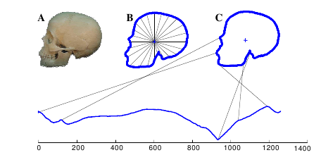
Each instance consists of a single time series (i.e. the problem is univariate) of equal length and a class label based on shape distinctions such as the presence and location of a notch in the arrow. The data set consists of 210 instances, by default split into 36 train and 175 test instances. We refer to the collection of time series as \(X\) and to the collection of class labels as \(y\).

Below, we store the data in a 3D dimensional (instance, variable, time point) numpy array for \(X\), and a one dimensional (instance) numpy array for \(y\).

For the single problem loader load arrow head, set the return type to numpy3D to store \(X\) in such a 3D ndarray. The data can also be returned in other formats, e.g., pd-multiindex (row-index hierarchical pandas), or numpyflat (2D numpy with rows=instances, columns=time points; alias is numpy2d). The full range of options are the Panel data format strings desribed in tutorial AA - datatypes and data loaders (see there).

# Imports used in this notebook
import matplotlib.pyplot as plt

from sktime.datasets import (
    load_arrow_head,
    load_basic_motions,
    load_japanese_vowels,
    load_plaid,
)

# Load all arrow head
arrow_X, arrow_y = load_arrow_head(return_type="numpy3d")
# Load default train/test splits from sktime/datasets/data
arrow_train_X, arrow_train_y = load_arrow_head(split="train", return_type="numpy3d")
arrow_test_X, arrow_test_y = load_arrow_head(split="test", return_type="numpy3d")
print(arrow_train_X.shape, arrow_train_y.shape, arrow_test_X.shape, arrow_test_y.shape)
plt.title(" First instance in ArrowHead data")
plt.plot(arrow_train_X[0, 0])

# Load arrow head dataset, pandas multiindex format, also accepted by sktime classifiers
arrow_train_X, arrow_train_y = load_arrow_head(
    split="train", return_type="pd-multiindex"
)
arrow_test_X, arrow_test_y = load_arrow_head(split="test", return_type="pd-multiindex")
print(arrow_train_X.head())

# Load arrow head dataset in nested pandas format, also accepted by sktime classifiers
arrow_train_X, arrow_train_y = load_arrow_head(split="train", return_type="nested_univ")
arrow_test_X, arrow_test_y = load_arrow_head(split="test", return_type="nested_univ")
arrow_train_X.iloc[:5]

# Load arrow head dataset in numpy2d format, also accepted by sktime classifiers
arrow_train_X, arrow_train_y = load_arrow_head(split="train", return_type="numpy2d")
arrow_test_X, arrow_test_y = load_arrow_head(split="test", return_type="numpy2d")
print(arrow_train_X.shape, arrow_train_y.shape, arrow_test_X.shape, arrow_test_y.shape)

# CAUTION:
# while classifiers will interpret 2D numpy arrays as (instance, timepoint),
#   and as a collection/panel of univariate time series
# all other sktime estimators interpret 2D numpy arrays as (timepoint, variable),
#   i.e., a single, multivariate time series
#   WARNING: this is also true for individual transformers, when outside a pipeline
#
# the reason for this ambiguity is ensuring sklearn compatibility
#   in classification, numpy 2D is typically passed as (instance, timepoint) to sklearn
#   in forecasting, numpy 2D is typically passed as (timepoint, variable) to sklearn

Some TSC datasets are multivariate, in that each time series instance has more than one variable. For example, the data [basic motions dataset] (https://timeseriesclassification.com/description.php?Dataset=BasicMotions) was generated as part of a student project where four students performed four activities whilst wearing a smart watch. The watch collects 3D accelerometer and a 3D gyroscope. Each instance involved a subject performing one of four tasks (walking, resting, running and badminton) for ten seconds. Time series in this data set have 6 variables.

# "basic motions" dataset
motions_X, motions_Y = load_basic_motions(return_type="numpy3d")
motions_train_X, motions_train_y = load_basic_motions(
    split="train", return_type="numpy3d"
)
motions_test_X, motions_test_y = load_basic_motions(split="test", return_type="numpy3d")
print(type(motions_train_X))
print(
    motions_train_X.shape,
    motions_train_y.shape,
    motions_test_X.shape,
    motions_test_y.shape,
)
plt.title(" First and second dimensions of the first instance in BasicMotions data")
plt.plot(motions_train_X[0][0])
plt.plot(motions_train_X[0][1])

Some data sets have unequal length series. Two data sets with this characteristic are shipped with sktime: PLAID (univariate) and JapaneseVowels (multivariate). We cannot store unequal length series in numpy arrays. Instead, we use nested pandas data frames, where each cell is a pandas Series. This is the default return type for all single problem loaders.

# loads both train and test together
vowel_X, vowel_y = load_japanese_vowels()
print(type(vowel_X))

plt.title(" First two dimensions of two instances of Japanese vowels")
plt.plot(vowel_X.iloc[0, 0])
plt.plot(vowel_X.iloc[1, 0])
plt.plot(vowel_X.iloc[0, 1])
plt.plot(vowel_X.iloc[1, 1])
plt.show()

plaid_X, plaid_y = load_plaid()
print(type(plaid_X))

plt.title(" Four instances of PLAID dataset")
plt.plot(plaid_X.iloc[0, 0])
plt.plot(plaid_X.iloc[1, 0])
plt.plot(plaid_X.iloc[2, 0])
plt.plot(plaid_X.iloc[3, 0])
plt.show()

Building Classifiers

We demonstrate the simplest use cases for classifiers and demonstrate how to build bespoke pipelines for time series classification.

It is possible to use a standard sklearn classifier for univariate, equal length classification problems but it is unlikely to perform as well as bespoke time series classifiers, since supervised tabular classifiers ignore the sequence information in the variables.

To apply sklearn classifiers directly, the data needs to be reshaped into one of the sklearn compatible 2D data formats. sklearn cannot be used directly with multivariate or unequal length data sets, without making choices in how to insert the data into a 2D structure.

sktime provides functionality to make these choices explicit and tunable, under a unified interface for time series classifiers.

sktime also provides pipeline construction functionality for transformers and classifiers that are specific to time series datasets.

Direct application of sklearn (without sktime) is possible via using the numpy2d return type for the time series data sets, and then feeding the format into sklearn:

from sklearn.ensemble import RandomForestClassifier
from sklearn.metrics import accuracy_score

classifier = RandomForestClassifier(n_estimators=100)
arrow_train_X_2d, arrow_train_y_2d = load_arrow_head(
    split="train", return_type="numpy2d"
)
arrow_test_X_2d, arrow_test_y_2d = load_arrow_head(split="test", return_type="numpy2d")
classifier.fit(arrow_train_X_2d, arrow_train_y_2d)
y_pred = classifier.predict(arrow_test_X_2d)
accuracy_score(arrow_test_y_2d, y_pred)

sktime contains the state of the art in time series classifiers in the package classification. These are grouped based on their representation. An accurate and relatively fast classifier is called ROCKET

from sktime.classification.kernel_based import RocketClassifier

rocket = RocketClassifier()
rocket.fit(arrow_train_X, arrow_train_y)
y_pred = rocket.predict(arrow_test_X)
accuracy_score(arrow_test_y, y_pred)

A state-of-art algorithm for time series classification is version 2 of the HIVE-COTE algorithm. HC2 is slow on small problems like these examples. However, it can be configured with an approximate maximum run time as follows (may take a bit longer than a minute to run this cell).

from sktime.classification.hybrid import HIVECOTEV2

hc2 = HIVECOTEV2(time_limit_in_minutes=1)
hc2.fit(arrow_train_X, arrow_train_y)
y_pred = hc2.predict(arrow_test_X)
accuracy_score(arrow_test_y, y_pred)

Most classifiers in sktime involve some degree of transformation. The simplest form is simply consisting of a pipeline of transformation (aka “feature extraction”) followed by an sklearn classifier.

The sktime make_pipeline utility allows to combine transformers and classifiers into a simple pipeline. The classifier pipelined can be an sktime time series classifier, or an sklearn tabular classifier. If an sklearn classifier, the time series are formatted as (instance, time index) formatted 2D array before being passed to the sklearn classifier.

In the following example, we use the tsfresh feature extractor to extract features which are then used in a (tabular, sklearn) random forest classifier. This can be done with the sktime’s make_pipeline utility as follows:

from sklearn.ensemble import RandomForestClassifier

from sktime.pipeline import make_pipeline
from sktime.transformations.panel.tsfresh import TSFreshFeatureExtractor

tsfresh_trafo = TSFreshFeatureExtractor(default_fc_parameters="minimal")
randf = RandomForestClassifier(n_estimators=100)
pipe = make_pipeline(tsfresh_trafo, randf)

pipe.fit(arrow_train_X, arrow_train_y)
y_pred = pipe.predict(arrow_test_X)
accuracy_score(arrow_test_y, y_pred)

In the following example, we pipeline an sktime transformer with an sktime time series classifier:

from sktime.classification.kernel_based import RocketClassifier
from sktime.pipeline import make_pipeline
from sktime.transformations.series.exponent import ExponentTransformer

square = ExponentTransformer(power=2)
rocket = RocketClassifier()
pipe_sktime = square * rocket

Under the hood, sktime’s make_pipeline utiltiy dispatches to right pipeline class that exposes different kinds of pipeline under the familiar sktime time series classification interface. In the above examples, these were SklearnClassifierPipeline (for sklearn classifiers at the end) and ClassifierPipeline (for sktime classifiers at the end):

pipe

pipe_sktime

Alternatively, the pipelines could have been constructed directly with the special pipeline classes for more granular control, see docstrings of the aforementioned classes for further options.

Pipelines can also be defined, even more concisely, by using the * dunder operator, which is a shorthand for make_pipeline. Estimators on the right are pipelined after estimators on the left of the operator.

from sktime.classification.kernel_based import RocketClassifier
from sktime.transformations.series.exponent import ExponentTransformer

square = ExponentTransformer(power=2)
rocket = RocketClassifier()
pipe = square * rocket
pipe

pipe.fit(arrow_train_X, arrow_train_y)
y_pred = pipe.predict(arrow_test_X)
accuracy_score(arrow_test_y, y_pred)

Using sktime pipeline constructs is encouraged above using sklearn Pipeline, as sktime pipelines will come with base class features such as input checks, input data format compatibility, and tag handling. However, sktime estimators are, in general, also compatible with sklearn pipelining use cases, as long as the sklearn adjacent data formats are being used, namely numpy3D or nested_univ. Conversely, sklearn native compositor elements will in general not be compatible with use of row hierarchical data formats such as pd-multiindex, and will not automatically convert, or provide sktime compatible tag inspection functionality.

Multivariate classification

Many classifiers, including ROCKET and HC2, are configured to work with multivariate input. For example

rocket.fit(motions_train_X, motions_train_y)
y_pred = rocket.predict(motions_test_X)
accuracy_score(motions_test_y, y_pred)
hc2.fit(motions_train_X, motions_train_y)
y_pred = hc2.predict(motions_test_X)
accuracy_score(motions_test_y, y_pred)

sktime offers two other ways of solving multivariate time series classification problems:

1. Concatenation of time series columns into a single long time series column via ColumnConcatenator and apply a classifier to the concatenated data,

2. Dimension ensembling via ColumnEnsembleClassifier in which one classifier is fitted for each time series column/dimension of the time series and their predictions are combined through a voting scheme.

We can concatenate multivariate time series/panel data into long univariate time series/panel using a tran and then apply a classifier to the univariate data.

from sktime.classification.interval_based import DrCIF
from sktime.transformations.panel.compose import ColumnConcatenator

clf = ColumnConcatenator() * DrCIF(n_estimators=10)
clf.fit(motions_train_X, motions_train_y)
clf.score(motions_test_X, motions_test_y)

We can also fit one classifier for each time series column and then aggregated their predictions. The interface is similar to the familiar ColumnTransformer from sklearn.

from sktime.classification.compose import ColumnEnsembleClassifier
from sktime.classification.dictionary_based import TemporalDictionaryEnsemble
from sktime.classification.interval_based import DrCIF

clf = ColumnEnsembleClassifier(
    estimators=[
        ("DrCIF0", DrCIF(n_estimators=10), [0]),
        ("TDE3", TemporalDictionaryEnsemble(max_ensemble_size=5), [3]),
    ]
)

clf.fit(motions_train_X, motions_train_y)
clf.score(motions_test_X, motions_test_y)

Background info and references for classifiers used here

The RocketClassifier

is based on a pipeline combination of the ROCKET transformation (transformations .panel.rocket) and the sklearn RidgeClassifierCV classifier. The RocketClassifier is configurable to use variants minirocket and multirocket. ROCKET is based on generating random convolutions. A large number are generated then the classifier performs a feature selection.

[1] Dempster, Angus, François Petitjean, and Geoffrey I. Webb. “Rocket: exceptionally fast and accurate time series classification using random convolutional kernels.” Data Mining and Knowledge Discovery 34.5 (2020) arXiv version

DrCIF

The Diverse Representation Canonical Interval Forest Classifier (DrCIF) is an interval based classifier. The algorithm takes multiple randomised intervals from each series and extracts a range of features. These features are used to build a decision tree, which in turn are ensembled into a decision forest, in the style of a random forest. The original version

[2] Matthew Middlehurst and James Large and Anthony Bagnall. “The Canonical Interval Forest (CIF) Classifier for Time Series Classification.” IEEE International Conference on Big Data 2020 arXiv version

The DrCIF adjustment was proposed in [4]

#### TDE he Temporal Dictionary Ensemble is a dictionary based classifier. The basic premise is to extract discrete patterns using a windowing and to count their occurence. Classification is based on these frequency histograms. TDE includes bigram frequencies, spatial pyramids and a Gaussian process based parameter search.

[3] Matthew Middlehurst, James Large, Gavin Cawley and Anthony Bagnall “The Temporal Dictionary Ensemble (TDE) Classifier for Time Series Classification”, in proceedings of the European Conference on Machine Learning and Principles and Practice of Knowledge Discovery in Databases, 2020. arXiv version

HiveCoteV2 (HC2)

The HIerarchical VotE Collective of Transformation-based Ensembles is a meta ensemble that combines classifiers built on different representations. Version 2 combines DrCIF, TDE, an ensemble of RocketClassifiers called the Arsenal and the ShapeletTransformClassifier. It is currently the most accurate classifier on the UCR and UEA time series archives.

[4] Middlehurst, Matthew, James Large, Michael Flynn, Jason Lines, Aaron Bostrom, and Anthony Bagnall. “HIVE-COTE 2.0: a new meta ensemble for time series classification.” Machine Learning (2021)

---

Generated using nbsphinx. The Jupyter notebook can be found here.